1 Summary
- The serial ODDS joint longitudinal and time-to-event model uses repeated six-minute walk test information to update a patient’s estimated transplant-free survival as new visits become available.
- The analysis included 449 patients, 2,341 6MWTs, and 208 deaths or lung transplantations.
- At any follow-up time, a 1-SD worse modeled ODDS value was associated with a 2.28-fold higher instantaneous rate of death or transplantation.
- Patient-level five-fold cross-validation showed consistently better discrimination for serial ODDS than for serial 6MWD alone. At the 1-year prediction start, ODDS AUCs were 0.784, 0.774, and 0.761 for the next 1, 2, and 3 years, respectively.
- Across all evaluated windows, ODDS also had lower overall prediction error by Brier score (0.113 to 0.214) than 6MWD (0.116 to 0.244). Pooled ICI ranged from 0.025 to 0.075 for ODDS and from 0.014 to 0.061 for 6MWD, with no systematic mean overprediction or underprediction for either model.
- Results were stable after reasonable changes to the association prior, baseline-hazard flexibility, and random-effects correlation.
- The model is internally supported, but prospective external validation is still required to evaluate model accuracy and calibration in other hospital systems and across disease processes.
Clinical interpretation: serial ODDS appears to capture clinically important changes that are not represented by walk distance alone.
2 Why Use a Joint Longitudinal and Time-to-event Model?
Repeated 6MWTs are not collected on a perfectly fixed schedule. Testing may stop because a patient becomes too ill, receives a transplant, dies, transfers care, or is otherwise lost to follow-up. This means that missing later measurements can be informative rather than random.
The joint model analyzes two linked processes at the same time:
- Longitudinal process: estimates each patient’s underlying ODDS trajectory from all available visits, allowing the starting level and rate of change to differ between patients.
- Time-to-event process: estimates the association between the patient’s current modeled ODDS value and subsequent death or lung transplantation.
- Shared patient effects: connect these processes so that the estimated trajectory and event risk are informed by the same latent disease course.
In practical terms: the model asks whether the patient’s ODDS level is worsening over time and how that updated disease course changes anticipated event-free survival. Joint modeling can reduce bias from dropout related to the modeled disease trajectory, but it cannot correct every source of missingness or unmeasured confounding.
3 Data and Model
| Item | Description |
|---|---|
| Patients | 449 |
| Primary endpoint events | 208 deaths or lung transplantations |
| Serial 6MWT observations | 2,341 |
| Primary longitudinal model | Linear time with a patient-specific random intercept and random slope |
| Survival association | Current fitted marker value linked to time to death or lung transplantation |
| Internal validation | Patient-level five-fold cross-validation; all visits from a patient remained in one fold |
Separate joint models were fit for ODDS and 6MWD. For the 6MWD comparison, distance was reversed before standardization so that a higher modeled value represented worsening in both models. The survival submodel contained the longitudinal marker but no additional clinical covariates. The log baseline hazard was represented with penalized quadratic B-splines.
The primary survival association used the current fitted marker value.
4 Reliability Checks
This summary focuses on checks that may affect confidence in the clinical interpretation.
4.1 Sampling Quality
The primary models used 4 independent chains with 20,000 iterations per chain, including 5,000 burn-in iterations. This produced 60,000 retained posterior draws per model.
| Model | Maximum key/derived R-hat | Minimum key/derived ESS | Result |
|---|---|---|---|
| ODDS | 1.003 | 1079 | Satisfactory |
| 6MWD | 1.005 | 587 | Satisfactory |
R-hat assesses whether independent chains converged to the same posterior distribution. Values near 1 are preferred. Effective sample size (ESS) reflects the amount of independent information in autocorrelated posterior draws. Larger values are preferred. Both primary models met the predefined criteria for the clinically important parameters and derived baseline survival.
4.2 Model Fit and Sensitivity
- Posterior predictive checks found no gross failure of the longitudinal or event submodels.
- The observed mean trajectories sometimes lay near the edge of the replicated range, and uncertainty widened late in follow-up as fewer observations remained. Late predictions (after long follow-up periods) should therefore be interpreted more cautiously.
- The ODDS association and prediction metrics changed very little with tighter or more diffuse association priors, a simpler baseline hazard, or independent random effects.
- All five ODDS cross-validation refits met the sampling criteria. Two 6MWD refits had weak estimation of the random-slope variance, while their survival associations and baseline-survival estimates remained stable.
5 Main Results
5.1 Association With Death or Lung Transplantation
| Model | Clinical worsening represented by 1 SD | Hazard ratio (95% credible interval) |
|---|---|---|
| ODDS | Higher ODDS by 1.23 raw-score points | 2.28 (1.91 to 2.72) |
| 6MWD | Lower 6MWD by 130 m | 1.82 (1.49 to 2.20) |
For ODDS, one standard deviation corresponded to approximately 1.23 raw-score points. A higher ODDS score represents clinical worsening. For 6MWD, one standard deviation corresponded to approximately 130 m of shorter walk distance.
5.2 Performance in Patients Not Used to Fit Each Fold
Patients, rather than visits, were assigned to five folds. Every visit from a patient stayed in the same fold, and marker standardization was estimated within each training fold. This prevented a patient’s measurements from contributing to both model fitting and testing in the same fold.
| Model | Prediction horizon | Target time from baseline | At risk at year 1 | AUC | Brier score | Pooled out-of-fold ICI |
|---|---|---|---|---|---|---|
| ODDS | Next 1 year | Year 2 | 328 | 0.784 | 0.116 | 0.025 |
| 6MWD | Next 1 year | Year 2 | 328 | 0.707 | 0.128 | 0.014 |
| ODDS | Next 2 years | Year 3 | 328 | 0.774 | 0.178 | 0.042 |
| 6MWD | Next 2 years | Year 3 | 328 | 0.676 | 0.200 | 0.030 |
| ODDS | Next 3 years | Year 4 | 328 | 0.761 | 0.206 | 0.029 |
| 6MWD | Next 3 years | Year 4 | 328 | 0.651 | 0.232 | 0.055 |
- AUC measures ranking: whether patients who experience an event are assigned higher risk than those who remain event free. A value of 0.5 is no better than chance and a higher value is better.
- Brier score measures overall probability error, combining discrimination and calibration. Lower is better.
- ICI is the average absolute difference between predicted and observed risk along a flexible calibration curve. Here, predictions from all held-out patients were pooled before the calibration curve was fitted. Lower is better.
Across the held-out folds, 328 patients remained alive and transplant free at the 1-year prediction start. The “next 1 year” prediction therefore targets year 2 from baseline, while the “next 3 years” prediction targets year 4 from baseline.
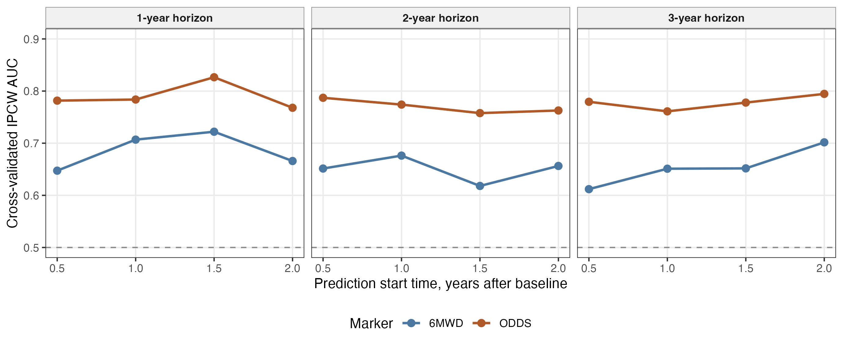
Figure 1. Patient-level cross-validated discrimination for serial ODDS and serial 6MWD.
Points and lines show the weighted mean IPCW time-dependent AUC across five held-out patient folds. Prediction start time is the point at which the patient’s available longitudinal history is used. Each panel shows the subsequent prediction horizon.
5.3 Calibration of Absolute Risk
| Model | Pooled ICI range | E50 range | E90 range | Interpretation |
|---|---|---|---|---|
| ODDS | 0.025 to 0.075 | 0.015 to 0.052 | 0.043 to 0.145 | No clear overprediction or underprediction |
| 6MWD | 0.014 to 0.061 | 0.006 to 0.062 | 0.033 to 0.126 | No clear overprediction or underprediction |
The Brier and ICI findings describe different properties. Serial ODDS had better discrimination and lower overall prediction error, while 6MWD had numerically lower pooled ICI. A model can therefore rank patients less accurately but still have average predicted probabilities that align closely with average observed risk.
- E50 is the median absolute difference between predicted and observed risk along the calibration curve.
- E90 is the 90th percentile of that difference and describes calibration error toward the less well-calibrated end of the prediction range.
At the 1-year prediction start, pooled ODDS ICI was 0.025, 0.042, 0.029 for the subsequent 1-, 2-, and 3-year horizons, respectively. Mean predicted and observed risks did not differ systematically, and all three calibration-slope intervals included the target value of 1.
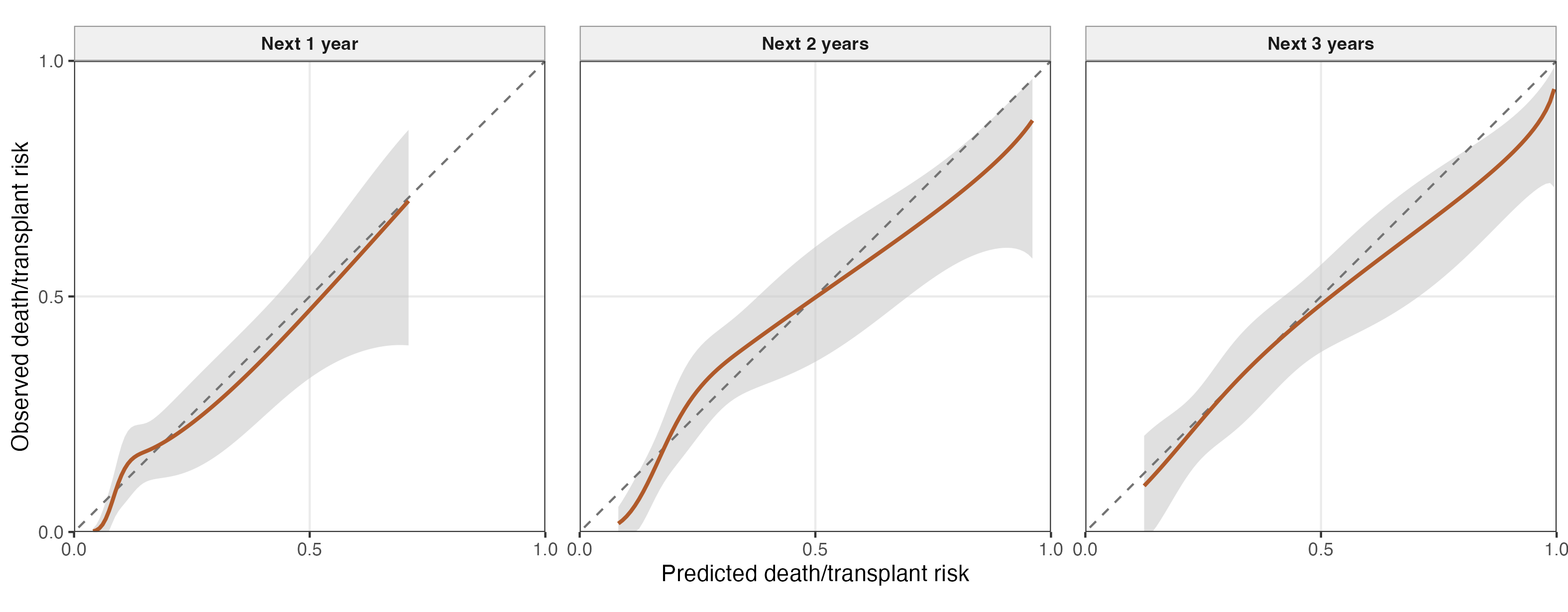
Figure 2. Pooled out-of-fold calibration of serial ODDS predictions beginning 1 year after baseline.
Solid lines compare predicted and observed death/transplant risk for the subsequent 1, 2, and 3 years. Grey regions are pointwise 95% intervals around observed risk, conditional on the saved held-out predictions. Dashed diagonals represent perfect agreement. Curves are displayed over the central prediction range used by the calibration model.
Across all 12 evaluations, pooled ODDS ICI ranged from 0.025 to 0.075 and E90 ranged from 0.043 to 0.145. There was no clear overall direction of mean calibration error. However, calibration slopes were below 1 in longer-horizon evaluations, indicating that these later probabilities warrant greater caution.
6 Robustness to Modeling Choices
| Analysis | ODDS hazard ratio (95% credible interval) | Apparent AUC | Apparent Brier | Apparent ICI |
|---|---|---|---|---|
| Primary model | 2.28 (1.91 to 2.72) | 0.789 | 0.177 | 0.042 |
| Tighter association prior | 2.27 (1.91 to 2.69) | 0.791 | 0.177 | 0.039 |
| More diffuse association prior | 2.28 (1.92 to 2.71) | 0.790 | 0.178 | 0.041 |
| Simpler baseline hazard | 2.28 (1.95 to 2.65) | 0.789 | 0.177 | 0.041 |
| Independent random intercept and slope | 2.29 (1.92 to 2.71) | 0.788 | 0.176 | 0.031 |
The estimated ODDS association remained approximately 2.27 to 2.29 across supported alternatives. Apparent AUC, Brier score, and ICI were also nearly unchanged. This stability indicates that the principal finding was not dependent on one narrow prior choice, the exact number of baseline-hazard spline segments, or estimation of the random intercept-slope correlation.
7 What These Results Support
Supported by the current analysis
- Serial ODDS is strongly associated with subsequent death or lung transplantation.
- Serial ODDS provides better internally validated risk ranking than serial 6MWD alone.
- Serial ODDS has lower cross-validated overall prediction error.
- Pooled calibration shows no systematic mean overprediction or underprediction, but some later, longer-horizon ODDS probabilities may be too extreme.
- The primary current-value joint model has satisfactory sampling diagnostics and no evidence of gross model failure.
- The main association and dynamic performance are stable across several modeling choices.
Not yet established
- External validity in a different health system or diagnosis (i.e., other fibrotic lung diseases or pulmonary disorders).
- Reliable performance far into follow-up or when serial testing becomes sparse.
8 Technical Specification
The longitudinal submodel was a Gaussian linear mixed-effects model with linear time, a patient-specific random intercept, and a patient-specific random slope. The event submodel was a relative-risk survival model for death or lung transplantation with a penalized quadratic B-spline baseline hazard and a current-value association with the fitted longitudinal marker.
The primary marker transformations were:
- ODDS: standardized marker =
(ODDS raw + 7.20477) / 1.22839. 6MWD comparison: standardized worsening marker =
(380.09623 - distance in meters) / 130.29415.
The primary current-value association prior was normal with mean 0 and SD 2. The random intercept-slope correlation used an LKJ prior with eta 3, and the baseline-hazard smoothing precision used a gamma prior with shape 5 and rate 0.5.
The analysis used R version 4.5.2 (2025-10-31) and JMbayes2 version 0.6.0. Dynamic AUC and prediction error used IPCW. Internal validation used the same patient folds for ODDS and 6MWD, with marker scaling re-estimated in each training fold. Calibration curves pooled predictions from all held-out patients and accounted for censoring through survival calibration models. Calibration-in-the-large used IPCW complementary-log-log models, and horizon-specific calibration slopes used Cox models. Patient-level bootstrap intervals resampled the pooled held-out predictions without refitting every fold model.
Exact patient-level dynamic prediction requires the fitted joint-model object or equivalent posterior draws together with the same preprocessing definitions. Saved fitted model objects are retained and can be made available upon reasonable request.
9 Conclusion
The serial ODDS joint model passed convergence, model-fit, sensitivity, and patient-level internal-validation checks. A worse current ODDS trajectory was strongly associated with death or lung transplantation and serial ODDS ranked future risk more accurately and had lower overall prediction error than serial 6MWD alone. At the 1-year prediction start, estimated and observed absolute risks were closely aligned, but ODDS model predictions may be too extreme in longer-horizon evaluations. Prospective external validation remains necessary to further assess model performance in other health systems and disease processes.